Cook's Theorem and You
It’s been almost a year since I read Computers and Intractability, one of the most well received books on the topic of computational complexity and NP-Complete problems. Since that time I’ve had two questions in the back of my mind related to this work. Firstly, how well do I understand the material I worked through and secondly what’s the applicability of this knowledge to someone in a software engineering role. I’m hoping to use these blog posts as a chance to address both of these questions.
For the first question I’m going to go with my favorite rule of thumb, you don’t understand something until you can explain it to someone else. I plan on trying to provide a basic explanation of the concepts covered in this book aiming to cover Cook’s Theorem and the 6 basic NP-Complete problems. To tackle the second question I will look through the list of NP-Complete problems in the index and see how many I can recognize in real world problems I’ve encountered.
Background
The core of this book is is about the class of the hardest problems in NP space that are classified as NP-Complete. We’ll discuss these terms in more detail below but it suffices to say that this is about recognizing types of problems that are intrinsically hard to solve, and so far no general polynomial time solutions exist. Instead we’re left looking for alternative strategies such as trying to find near optimal solutions or solving sub sections of the problem. To start with though we need to discuss how we can classify problems.
Decision Problems and the Languages that love them
Much like you might expect, decision problems are questions where the answer is simply yes or no. For example, can I get from Node A to Node B in a graph in fewer than 3 steps? Decision problems are useful to look at for two reasons, firstly they are directly tied to optimization problems in a natural manner. It’s easy to see how the optimization problem of finding the fewest steps from Node A to Node B must be at least as hard as the decision problem above. Secondly decision problems have a natural formal counterpart called a Language. Let’s look at a simpler decision problem.
For a positive integer N: Is there a positive integer m such that N = 4m
We can understand that this question is simply asking if N is evenly divisible by 4. In order to have a Language we need an alphabet, which means we need a uniform way to encode our given problem. there are plenty of ways we could encode this problem, think about making a file format for storing questions of this form. For an example I’m going to make a slightly more complicated format of [Length of N in binary encoding]-[N in binary] instead of the just recording the number in binary to make it easier to illustrate some later points.
Sample #1
4-1100
This is one reasonable encoding (e) for our problem (P). An encoding is reasonable if it is concise and decodable. By concise we mean that we avoid so much padding that a question that was polynomial time starts taking exponential time due to the length of the encoding. Decodability similarly means we can get back from any encoding to our original component in polynomial time as well.
We can see that the set of characters used by our encoding scheme looks like this {0-9,-}. Now let us look at all possible strings composed only of these characters, so in addition to our encoding above we also have strings like this.
Sample #2
4-1101
Sample #3
12-15-9
Now where do Languages come in? We can see that our infinite set of strings splits into three groups. Strings that aren’t valid encodings of our problem (#3). Strings that are valid encodings of an instance of our problem whose answer is No (#2). This leaves our Language (for this e and P); the strings that are valid encodings whose answer is Yes (#1).
So now that we know what know what a Language for our encoding is, what does that get us? We can show that anything that holds for L(e,P) holds for any other L(e’,P) as long as both encodings meet our reasonable requirement. This lets us make our proofs become encoding independent. Secondly Turing machines that recognize languages provide us with a formal way to classify our problems by going from the Original Problem -> The Language comprised of ‘Yes’ encodings of our problem -> The run time of the Turing Machine that recognizes the language.
Turing Machines, P, and NP
Some people may remember the standard one tape deterministic turing machine (DTM) from classes in school. It has a single read/write head and an infinitely long tape that it operates on. The DTM is controlled by a state machine that takes two inputs, the current state of the machine and the symbol under the R/W head. Based on those two inputs it determines the new state, picks a symbol to write out into the current space, and then moves the head one space left or right. One of simple tasks you can put a DTM towards is recognizing a Language, it’s relatively simple to see how a Turing machine could recognize our divisible by 4 problem. It simply needs to move the head to the right until it reaches a blank character, then move backwards two steps checking for zero. A DTM can perform the same computations as any other computer, and while they’re slower they are within polynomial time. Consequently our chosen computation model doesn’t affect our findings. We can now separate our proofs from both the encoding and the underlying hardware. We’ll continue using DTM’s as they are a convenient baseline for defining time complexity.
We say that a Language (and thus a problem) belongs to class P if there is a polynomial run time DTM program which recognizes the Language. Most of us will just boil this down in our minds to ‘a computer algorithm can solve this problem in polynomial time’ which is sufficient for our purposes, but we’ll want to use the slightly deeper understanding we now have to define the class NP. We’ve already looked at problems that can be solved in polynomial time, but now lets look at problems where we can verify a possible solution in polynomial time (NP). We can understand that some problems which don’t appear to be easily solvable (P) are at least easily verifiable (NP). The Traveling Salesman Problem (TSP) is an optimization problem, which as we discussed earlier means it has a decision problem version we can examine more closely.
For a set of cities with known distances between every pair of cities,
is there a tour that visits all cities and ends back at the start point
with a total distance <= B
You can take my word that there is no easy polynomial solution to this decision problem, however it should once again be easy to see how verification of a potential answer could be done in polynomial time. The tour needs to start from the start point, visit each node at least once, and end at the start point. If that criteria is met and the total distance traveled is <= B then the answer is yes.
Now how can we take advantage of a problem with easily verifiable solutions? Enter the Non Deterministic Turing Machine (NDTM). This turing machine is a pure thought experiment, but it lets us set a bound for computational complexity. An NDTM is very similar to a DTM with one minor modification. A second write only head writes out a random string from the alphabet onto the tape in place of the normal input, then the machine starts using its R/W head and state chart to move through the input tape like any other DTM. Instead of only having a single computation path we now have one for every possible input path occurring at the same time, and since each verification takes only polynomial time this NDTM is capable of ‘solving’ our decision problem in polynomial time. Now as I pointed out earlier, this is a thought experiment designed to capture the fact that a problem is verifiable in polynomial time, not actually solving it. We can now formally say that the class NP consists of Languages for which there is a polynomial time NDTM program which recognizes the Language.
It should be fairly straightforward to see that NP contains P as you could find a NDTM that ignores the provided potential solution and solves the problem (which can be done in polynomial time). It’s important to note at this point that the assumption P != NP is one of the outstanding questions in computer theory. However almost all of the study in the area is based off of the assumption that P != NP( That is that there are problems in NP which don’t have an easy solution), if you can prove otherwise you shouldn’t be reading this.
You NP-Complete Me
Before we dig out the formal definition of NP-Complete we need to understand how we can compare decision problems. One of the most powerful tools to do this is the polynomial transformation of one Language to another. Let’s look at the Hamiltonian Circuit decision problem. A graph is said to have a Hamiltonian circuit if there is a traceable cycle that visits every vertex exactly once. We can see that this problem seems somewhat similar to the TSP mentioned earlier. In order to show a formal transformation from HC to TSP we have to do two things. First we have to specify a function that maps an instance of the HC problem into the TSP (in polynomial time), and then show that a potential answer X to the HC question is yes if and only if it also provides a yes answer to the transformed TSP.
The transformation is actually fairly simple, assume we are given an instance of the HC problem, a graph (G) made up of vertexes (V) and edges (E), and that the number of vertexes is m. We simply create a TSP where the cities are identical to our V, and the distance between any two cities is 1 if that edge exists in E, and 2 otherwise. We then finish by setting the tour length cutoff (B) to equal the number of vertexes and cities(m). You can see that this transformation is applicable in polynomial time as we only need to step through the edges (m*(m-1)/2) and check for their existence in E.
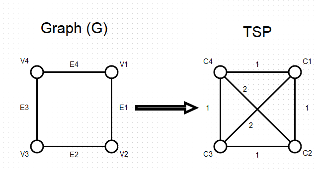
Now we need to show that our graph has a Hamiltonian circuit if and only if their is a tour of the city with length no more than B. Assume that N = [v1, v2, … vm] is a Hamiltonian circuit of G, then it must also be a tour of the city and its length is B as each edge has a distance of 1. Conversely if N is a tour with a length no more than B, we know that the number of distances summed is m, B/m = 1 indicates that the length of each inter-city distance must be 1, meaning that every path taken was an edge in E, so by definition it’s a Hamiltonian Circuit.
So what does knowing that HC transforms to TSP provide us? We can show that if the TSP can be solved by a polynomial time algorithm then so can HC. This means that the TSP problem is at least as hard as the HC problem. Combining this understanding with another Lemma showing that if A transforms to B, and B transforms to C, then A transforms to C gives us the tools to start classifying the difficulty of problems within NP. This is where NP-Complete comes in.
The formal definition of an NP-Complete Language (L) is that it must be in NP (polynomial time verifiability of an answer) and all other Languages (L’) in NP can transform into L.
Combining this definition with what we just said about the ordering implied by transforms we can see that an NP-Complete problem must be the hardest problem in NP as if any problem in NP-Complete can be solved in polynomial time then all problems in NP can be similarly solved.
We are now ready to combine the final Lemma needed to populate NP-Complete. If L1 and L2 belong to NP, and L1 is NP-Complete, and L1 transforms to L2, then L2 is also NP-Complete. This is straight forward as we know L2 belongs to NP, and since any L’ transforms to L1 by the definition of NP-complete, L’ also transforms to L2 due to the earlier transitivity we discussed.
Now we just need an initial NP-Complete problem and we can prove any other problem is NP-complete once we’ve shown it exists in NP and that our NP-Complete problem transforms into it. This is where Cook’s Theorem gets the ball rolling by being the first proof of an NP-Complete problem, however this post is already running long so come back next time for Cook’s Theorem!